![]()
Following the August, 24 MW 6.0 earthquake, INGV, in collaboration with the Ufficio Rischio Sismico e Vulcanico of the Dipartimento Protezione Civile (DPC) and the Servizio Geofisica of the Istituto Superiore per la Protezione e la Ricerca Ambientale (ISPRA), started a detailed ground deformation monitoring in the epicentral area using the Global Positioning System (GPS) technique (INGV Working group “GPS Geodesy”, https://doi.org/10.5281/zenodo.61355). Several GPS stations have been installed on benchmarks belonging to the INGV CaGeoNet network (Galvani et al., 2012) and to the Istituto Geografico Militare network (IGM, www.igmi.org) (Fig. 2.7.1). Moreover, a new INGV-RING continuous GPS station has been monumented at Arquata del Tronto (ARQT). After the Mw=5.9 October 26 earthquake, we installed GPS instruments on a few other IGM benchmarks that were already re-occupied during the 1997 Umbria-Marche seismic sequence (see Anzidei et al., 2008). Not all the stations were operative simultaneously, because of electrical power problems and receivers movements over the different campaign benchmarks. Data from continuous and survey-mode GPS stations operating during the Mw=5.9 October 26 and Mw=6.5 October 30 earthquakes have been downloaded in the following hours or days, and processed by the three INGV-CNT GPS data analysis centers, using three different analysis software (GAMIT/GLOBK, GIPSY and BERNESE), and later combined in a single, consensus, co-seismic solution, obtained with the goal of minimizing the possible systematic errors present in the individual solutions (es., Devoti, 2012; Serpelloni et al., 2012). Figure 2.7.1 shows the measured co-seismic displacements for the Mw=5.9 October 26 earthquake and the distribution of the different GPS stations operating in the epicentral area from August, 24. Figure 2.7.2 shows the co-seismic displacements observed for the Mw=6.5 October, 30 event (note the different vector scales in the two figures). In both cases, the co-seismic displacements have been estimated starting from the position time-series, as the difference between the average position for the 10/17/2016-10/26/2016 interval and the position at the 10/27/2016 for the October, 26 earthquake, and the average position for the 10/27/2016-10/29/2016 interval and the position at the 10/30/2016 for the October 30, earthquake.
For the October 26 event, the maximum horizontal co-seismic displacements have been observed at the stations FIAB (3.1 cm towards north-east) and CAMP (2.7 cm towards south-west), whereas SLLI has shown the largest vertical motion, with a subsidence of about 1.7 cm. As regard the October, 30 event, the largest horizontal co-seismic displacements have been measured at the stations VETT (Mnt. Vettore) and MSAN, with 38.3 cm toward north-east and 26 cm toward south-west, respectively. The largest vertical co-seismic displacements, instead, have been observed for the stations ARQT, RIFP and MSAN, with a subsidence of 44.6, 26.1 and 17.1 cm, respectively. The GPS station at Mnt. Vettore (VETT), instead, showed an uplift of 5.5. cm.
Figure 2.7.3 shows the results of a preliminary co-seismic slip model for the Mw=6.5 October, 30 earthquake, obtained from the inversion of the displacements shown in Fig. 2.7.2. The inversion has been performed using a half-space elastic dislocation modeling approach, accounting for the topography of the area. In Fig. 2.7.3 the magenta rectangles show the coseismic faults obtained from non-linear inversion of the August, 24 and October, 26 events. In the slip inversion, instead, the fault plane for the Mw=6.5 event has been fixed (length = 40 km, width = 18 km, dip= 45° e strike = 160°) and the slip distribution has been estimated on a discretized fault plane with patches of variable dimension (1×1 km down to 3.5 km of depth, and 3.5.×3.5 km for deeper patches) using the approach described in Cheloni et al. (2010). This slip model, which must be considered preliminary, shows a shallow slip concentration (with a maximum slip value of 2.5 m), corresponding to a Mw = 6.5.
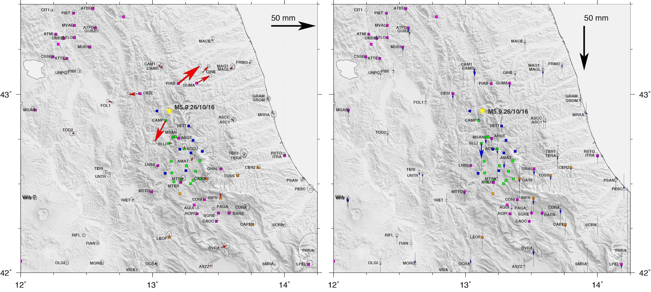
Figure 2.7.1: Map of GPS horizontal (red arrows) and vertical (blue arrows) co-seismic displacements for the October, 26 events obtained from the combination of three independent geodetic solutions. The white squares show the position of continuous GPS stations, the magenta squares show the position of the INGV-RING (doi:10.13127/RING) continuous GPS stations. The orange square shows the continuous GPS stations managed by DPC and ISPRA. The green and blue squares show the benchmarks of the CaGeoNet and IGM networks re-occupied after August, 24.
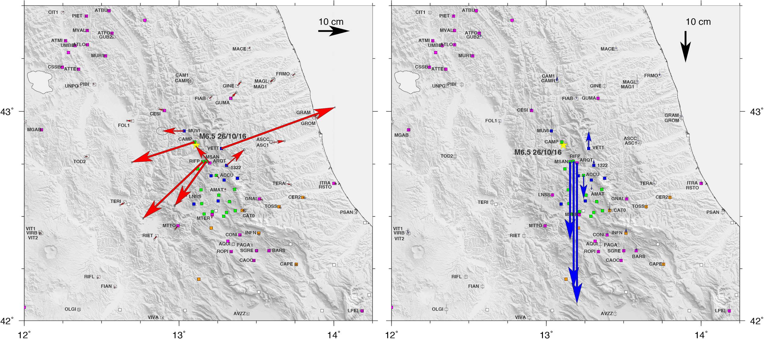
Figure 2.7.2:. Map of GPS horizontal (red arrows) and vertical (blue arrows) co-seismic displacements for the October, 30 event obtained from the combination of three independent geodetic solutions. The white squares show the position of continuous GPS stations, the magenta squares show the position of the INGV-RING (doi:10.13127/RING) continuous GPS stations. The orange squares shows the continuous GPS stations managed by DPC and ISPRA. The green and blue squares show the benchmarks of the CaGeoNet and IGM networks re-occupied after August, 24.
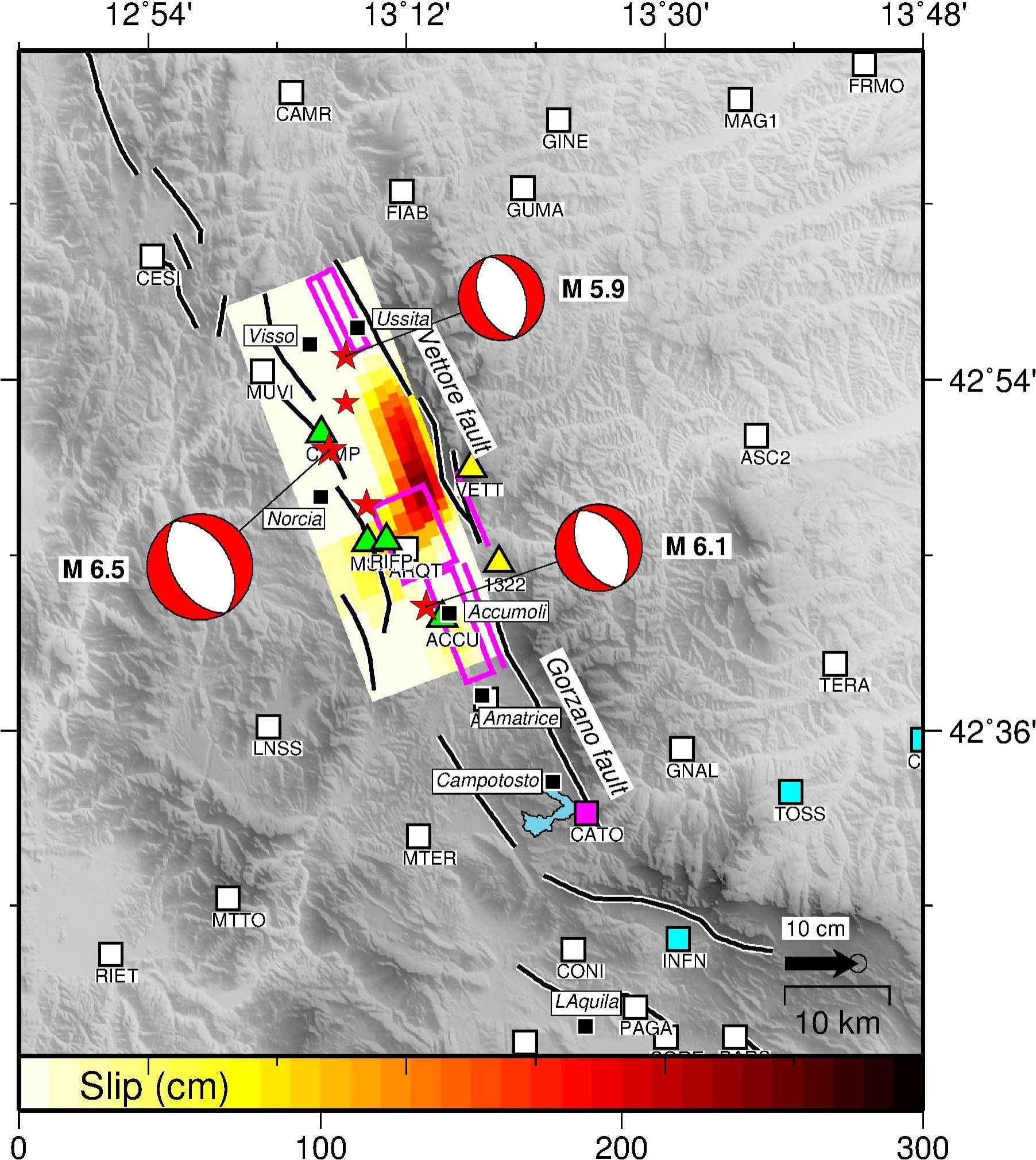
Figure 2.7.3: Co-seismic slip model for the Mw6.5, October, 30 event, obtained from the inversion of GPS displacements shown in Fig. 2.7.2. The magenta boxes show the co-seismic faults obtained from the non-linear inversion of GPS displacements for the August, 24 and October, 26 events.
Additional continuous GPS data have been provided by the Regione Abruzzo GNSS network (http://gnssnet.regione.abruzzo.it), the Regione Lazio GNSS network (http://gnss-regionelazio.dyndns.org), the ItalPos GNSS network (http://it.smartnet-eu.com), the NetGeo GNSS network (http://www.netgeo.it), the Regione Umbria GNSS network (http://www.umbriageo.regione.umbria.it), the ASI-Geodaf network (http://geodaf.mt.asi.it) and the Euref network (http://www.epncb.oma.be).
The tables reporting the coseismic offsets for the October, 26 and 30 events are available at the following links:
ftp://gpsfree.gm.ingv.it/amatrice2016/static/Cosismico_26Oct2016_GPS_GdL_V1.dat
ftp://gpsfree.gm.ingv.it/amatrice2016/static/Cosismico_30Oct2016_GPS_GdL_V1.dat
The table reports the co-seismic displacements (in mm) estimated for cGPS station around the epicentral area (up to 100 km of distance). The first column indicate the cGPS station name (site ID); lon. Is the longitude (°E), lat is the latitude (°N), Hei is the station height (in meters), East, sigE, North, sigN, Up, sigUp are the east, north and vertical co-seismic displacements and uncertainties, in mm.
References
Devoti, R. (2012), Combination of coseismic displacement fields: a geodetic perspective, Ann Geophys-Italy, doi:10.4401/ag-6119.
Galvani, A., M. Anzidei, R. Devoti, A. Esposito, G. Pietrantonio, A. R. Pisani, F. Riguzzi, and E. Serpelloni (2013), The interseismic velocity field of the central Apennines from a dense GPS network, Annals of Geophysics, 55(5), doi:10.4401/ag-5634.
Serpelloni, E. et al. (2012), GPS observations of coseismic deformation following the May 20 and 29, 2012, Emilia seismic events (northern Italy): data, analysis and preliminary models, Annals of Geophysics, 55(4), doi:10.4401/ag-6168.
Cheloni, D. et al. (2010), Coseismic and initial post-seismic slip of the 2009 Mw 6.3 L’Aquila earthquake, Italy, from GPS measurements, Geophys. J. Int., 181, doi:10.1111/j.1365-246X.2010.04584.x.